Résumé
L’auteur applique les techniques informatiques au domaine de la géo-archéologie, en combinant dans un SIG des données géomorphologiques, environnementales et archéologiques. L’objectif principal est le repérage du cadastre romain dans la région de Béziers, dans le Sud de la France. Différentes techniques (SIG, GPS, télédetection et images numériques) sont employées pour la collecte, le stockage, la numérisation et l’analyse des données géo-archéologiques. L’auteur utilise un SIG pour exploiter la base, analyser les données spatiales et quantitatives, et générer une image numérique de l’élévation du terrain. La base permet de reconstituer trois hypothèses de cadastres romains pour la région de Béziers, établies selon des critères dorientation et de distance des axes, et d’en choisir une.
Abstract
The study focuses on the application of computing elements in the field of geoarchaeology. Emphasis is placed on the meaningful combination of geomorphological and environmental data along with archaeological features within Geographic Information Systems. Principal objective was the identification and the modeling of possible Roman cadastres in the area of Béziers, in southern France. For this purpose numerous technologies have been applied; GIS, GPS, Remote Sensing techniques and Digital Image Processing methods were used for the collection, storage, digitization and analysis of geoarchaeological data. Geographical Information System (G.I.S.) was used for the processing of primary data, the production of secondary information layers, the development of the digital elevation model and its derivative files and, in essence, for the spatial and the quantitative analysis of the data. The research concluded at 3 potential Roman cadastre grids establishing orientation and distance of axes as main criteria. Further processing of the data concluded in one final Roman cadastre grid for the area of Biterrois in France.
Table of contents
Introduction
The area of study, the Sud Biterrois of Southern France, is a coastal region where the flow of three rivers result in a gentle relief and in the prevailing alluvial deposits. This combination is the reason that the fertile plain was inhabited from very early times; the first settlements date back to the Neolithic times. The region underwent rapid development during the Roman colonization dated back in 36 B.C.
The following lithologic formations are covering the area: a) Alluvial, b) Marles, c) Limestones d) Limestones, Conglomerates, Sands, e) Conglomerates, f) Dunes and g) Basaltic, Volcanic. Alluvials and marles represent the 61% of the total area, while basaltic and volcanic formations only represent the minimum percentage of 1%.
The map of figure 1 depicts that the terrestial deposits surpass the rest of the formations. The main proportion of limestones exists in the southern part of the study area, while in the eastern part volcanic and basaltic formations are met. The dunes are located along the coastline and present two propagations to the inlands.
The aim of the study is to record and analyze the physicogeographical, geomorphological, geological and archaeological characteristics of the area with the use of modern technologies.
With the intention of the most flexible combination of data, the best tool is the one combining the geographical along with the descriptive information. The combination of the geographic location of the settlements and their historic background together with the conjunction of cadastres’ metrologic data with the topographic, geological and geomorphological information are the key elements of the spatial analysis of the Roman colony regarding the distribution of settlements and the creation of the cadastral system.
The tool that corresponds perfectly to the aforementioned needs is the Geographic Information System. Having imported all the necessary data in the GIS, the user has the potential of analyzing one feature in combination with the others.
To achieve the most meaningful results concerning the relationship of geographical, geomorphological, geological and archaeological data of the area, a quantitative, a spatial and a combinatory analysis took place. Secondary information layers have been created on the basis of primary data and, then, several thematic maps have been produced such as the map of topographic inclinations, the map of the most possible Roman cadastre, as well as combinatory maps such as the map depicting the morphological inclinations, the drainage basin or the lithology of the area in correlation with the possible lines of Roman cadastre.
Methodology
In view of the research’s objectives, the collection, the recording and the digitalization of physicogeographic, geological and archaeological data of the area of Biterrois took place within GIS environment (Aronoff, 1989; Burrough, 1983; Chrisman, 1987; Clarke, 1990; Dangermond 1982; Demers, 1997; Korshkariov et al, 1989; MapBasic, 1999; MapInfo Professional, 1998; Marble & Peuquet, 1983; Marble et al, 1990; Rhind, 1988; Rhind, 1992; Snyder, 1988). Primary data was mainly derived from fieldwork, from the photointerpretation of aerial photographs (Avery, 1973; Evelpidou, 2001; Tomlinson, 1984), from the SPOT satellite image (Lillesand & Kiefer, 1995) and from analogue maps. The digital data was quantitatively and spatially analysed through GIS software and methods of photogrammetry.
Having recorded and stored in the geographic database the exact location of the archaeological settlements of the area of Biterrois with the use of GPS (Dana, 1997; Dana, 1998a;Dana, 1998b; Dana & Bruce, 1990; Kaplan, 1996) and GIS corresponding thematic maps were created. Furthermore, the recording of the precise location of the possible linear elements of the Roman cadastre took place on the basis of the results of photointerpretating the satellite image and the aerial photographs of the area, of fieldwork (with combinatory use of GPS and GIS) and of the studying the maps. In order to accomplish precision of data, the registration of maps and of the rectified satellite image was undertaken, while the stereoscopic observation of the aerial photographs via specific photogrammetric software was equally significant. The mapping of the geomorphologic characteristics was accomplished via fieldwork and via the photointerpretaion of the compliant aerial photographs. Photointerpretation was elaborated directly from the computer’s monitor using specific stereoscopic glasses of liquid crystals. This method enables actual navigation over the virtual relief of the region.
Primary data was, further, elaborated in order to derive secondary information layers such as morphological inclinations, combinatory output maps, tables and diagrams to be, afterwards, analysed.
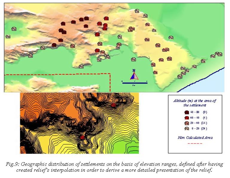
For the 3-dimensional analysis of input data, various algorithms and models for 3-variable grids have been used (Akima, 1978, Fotheringham & O’Kelly, 1989, Goldberger, 1962). For the manipulation of altitude data and the creation of the Digital Terrain Model – DTM, an information layer with points of absolute altitudes covering the whole area was initially created on the basis of primary information layers of elevation contours and altitude points. In order to create the Digital Elevation Model – DEM, all the elevation contours were converted to the points constituting the lines. The altitude values ascribed to the points were the altitude values of corresponding precedent lines. It is common place that the more elevation points available, the most credible and precise the derivative DEM is. A Data Aggregation Algorithm was applied to the elevation points information layer, in order to remove all the redundant points, whose value was already known from neighbour points. Afterwards, the algoritm “Triangulation with Smoothing” was applied for the creation of DEM (Fig.9) (Vertical Mapper, 1999). This algorithm is apt for the needs of the case study, because it is prerequisite for all the elevation points to directly contact the output surface and the specific algorithm, additionally, results in a smooth and continuous surface.
The derivative DEM was used for:
- The elaboration of 3-dimensional representations.
- The queries regarding altitudal information along linear elements (cross sections).
- The queries regarding altitudal information of selected points on the surface (point inspection) and selected regions in prospect of statistical analysis of elevation values.
The application of the aforementioned methods in the area of study enabled the automatic calculation of the morphologic inclination of every pixel of the map and, consequently, of every point correspondent to the settlements’ locations, identified and mapped during fieldwork. The topographic inclinations of the area have been calculated within the GIS via the following form and confirmed via the photointerpretation of the compliant aerial photographs.
![]()
where:
ΣL is the total length of contours falling within each single pixel
i is the interval of the contours
E is the area of each pixel
Resultanlty, a grid of 5 534 pixels was produced. Each pixel’s area equals 300x300m, except those falling onto the coastline and, in consequence, their area is defined by the coastline.
Having applied this methodology, the contours of the study area have been recreated in a more detailed interval value (1m) than the initial one available from the topographic maps (5m) (Fig. 9).
A more detailed analysis and an optical presentation of both the linear elements and the settlements’ sites in relationship to the relief was, therefore, feasible. The algorithm of creating cross sections was applied in order to derive the most accurate analysis of the physicogeographic characteristics in conjuction to the settlements.
Finally, one of the research’s objectives was the study of the settlements’ relationships concerning intervisibility in view of a better understanding of their selection and their geographic distribution (Wastson, 1992). For that reason, a series of algorithms have been applied and resulted in the following analyses:
- Quantitative analysis of the area’s visibility: Through this analysis it is feasible to find out if a point on the map is visible or not from a pre-selected point of view. Figure 11 depicts, in a quantitative way, the visibility of the area from the highest point (point A) of the study area. The different colours represent the high that may descrese or increase to every pixel of the area in order to remain visible from the pre-selected point A.
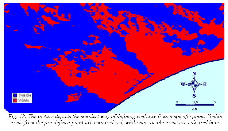
- Logical analysis: This analysis provides a Yes/No answer; that is if specific points on the map are visible (Y) or not (N) from a specific point. The map (Fig. 12) presents only 2 colours for the whole area depicting if the specific points are visible or not from Beziers area.
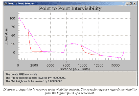
- Visibility analysis between 2 specific points. This analysis was applied for all the points representing Roman sites (data recorded during fieldwork). There is a line connecting the points of controlling visibility; parts of that line are represented by different colour whether this part is visible or not from the point of view. Figure 13 indicates the visibility of every site from Beziers area. Parts of the line connecting Beziers with each settlement are coloured either green or red indicating if they are visible or not from Beziers. The algorithm provides the results of the visibility analysis as a graph as well (Diagram 1).
Case study
Low values of average % inclinations characterize the biggest part of the area. The spatial analysis proved that the highest values are located in the southeastern part of the area and coincide with areas with carbonate rocks (Fig. 2).
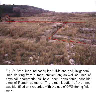
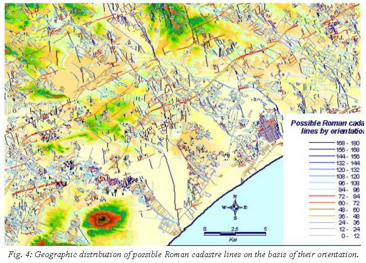
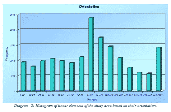
The orientation of every linear element corresponding to potential axis of the Roman cadastre (Fig. 3) was calculated with the algorithm ‘Cadastre Grid’ (Vassilopoulos, 1999). The thematic map of figure 4 depicting lines with different colours depending on the range of azimuthial orientation they fall within, was afterwards created. Fifteen ranges of azimuthial orientation have been defined and the number of lines falling within each range is presented in table 1. The histogram of the distribution of linear elements of the area (Diagram 2) shows that the prevailing orientation is 358ο and the vertical 88ο that conforms to Roman cadastre A according to Clavel-Leveque (2002). The analysis of the average distances of lines resulted in the following predominant distances of 702 m, 707 m and 803 m.
| Ranges | Frequency |
|---|---|
| 0-12 | 941 |
| 12-24 | 802 |
| 24-36 | 981 |
| 36-48 | 1.050 |
| 48-60 | 990 |
| 60-72 | 923 |
| 72-84 | 1.103 |
| 84-96 | 2.384 |
| 96-108 | 1.746 |
| 108-120 | 1.455 |
| 120-132 | 1.075 |
| 132-144 | 754 |
| 144-156 | 587 |
| 156-168 | 570 |
| 168-180 | 1.413 |
Applying the algorithm‘Cadastre Grid’ (Vassilopoulos, 1999), three potential digital models of Roman cadastres have been produced. The prevailing orientation is stable for all the models that are differentiated regarding the distances of the lines (702m, 707m and 803m). For the creation of the possible cadastres’ models three parameters have been considered:
- The distance between 2 successive axes of the cadastre
- The orientation of the axes
- The tolerance
The two first parameters are pertaining to the dimensions of the grid, while the third one refers to the width of every line of the grid; if any axis falls within this width, it is considered to belong to the specific grid.
Possible errors caused during digitization of axes and during the registration of maps, satellite images and aerial photograpshs are, thus, considered. Moreover, this methodology takes into account the width of the axes, important factor given that axes represent roads.
The output digital grids were, then, moved onto the area along the x and the y axis gathering every time the lines falling within each grid. In addition, lines shaping possible centuries were recorded in the GIS database for every grid. The grid with 707m distance of axes and orientation 358ο assigned the biggest number of lines (765) falling within the digital grid and the biggest number of possible centuries (44). The aforementioned model of cadastre is in compliance with results already published (Clavel-Leveque, 2002) and regard Roman cadastre A of the study area.
The map of figure 5 shows the prevailing grid with possible lines of Roman cadastre and possible centuries. With concern to the Roman cadastre of the area of Beziers numerous researches have been undertaken in the past (Clavel-Lévêque, 1992; Clavel-Lévêque, 1993; Clavel-Lévêque, 1983a & b; Clavel-Lévêque, 1988; Clavel-Lévêque, Lorcin & Lemarchand, 1983; Chouquer & Clavel-Lévêque, 1990; Clavel-Lévêque, 1993). Given that the Roman cadastre often followed “the orientation” defined by physical parameters, such as the morphology of the area or the drainage basin, a relative analysis of the orientation of the possible lines of Roman cadastre and the orientation of branches of drainage system took place. Hence, the statistical analysis concluded that the predominant orientation of the drainage system falls within the range of values 80-100ο (Fig. 6) and coincides with the prevailing orientation of the possible lines of the Roman cadastre.
The combinatory analysis of the possible Roman cadastre’s lines and of the lithology of the area of Beziers aimed at finding the lithologic formation that gathers most of the lines. The statistical analysis of lines in relation to the lithology attributed the biggest proportion of lines on alluvial and marles; this is understandable since the greates part of the area (60,9%) is covered by those formations. Both the alluvial deposits and the marles, due to their vulnerability, cause a gentle relief in favour of agricultural activities.
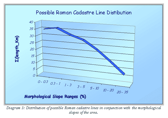
Morphologic inclinations have been analysed with the same methodology as the lithological formations (Diagram 3).
The analysis of the locations of the settlements in combination with the physicogeographic, geomorphologic and lithologic characteristics of the area was undertaken within the corresponding information layers having produced in the GIS by applying Simple Query Language (SQL). The diagram 4 demonstrates that the orientation of the possible lines of Roman cadastre coincides with the main physicogeographic axes and, especially, with the ones of the drainage system.
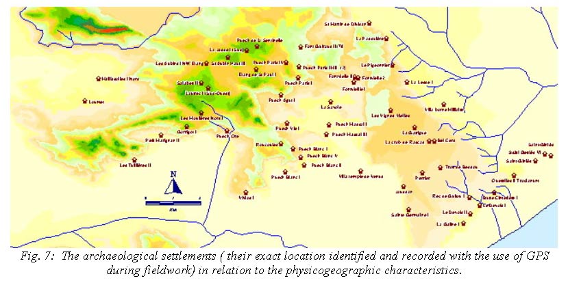
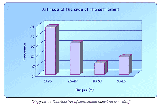
The analysis concluded that 24 settlements, the biggest proportion of sites (43,6%), are located at an elevation of 0-20m, 15 settlements (27,3%) are at an altitude of 20-40m, 7 settlements (12,7%) at 40-60m, 9 settlements at 60-85m (Fig. 7), while there is no settlement at the elevation ranges 35-40m and 60-65m (Diagram 5).
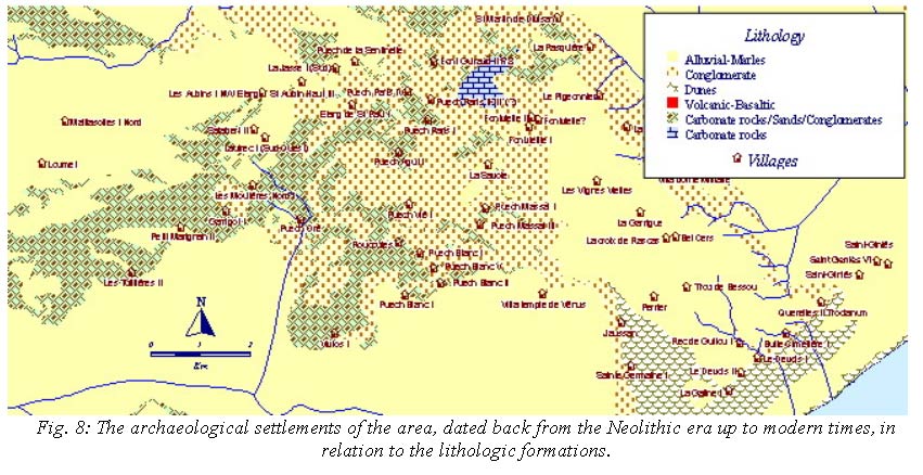
Regarding the relationship of the settlements with the lithological characteristics of the area, 22 settlements (40% of the total settlements) are located on Alluvial – Marles, 16 settlements (29,1%) on Conglomerates, 2 settlements (3,6%) on dunes and 15 settlements (27,3%) on Carbonates /Sands /Conglomerates, while there is no settlement on volcanic-basaltic or carbonate rocks (Fig. 8).
Spatial and quantitative analysis of the settlements in combination with the chronological periods of habitation took place along with the visibility analysis. In the beginning of the 1st century B.C, the settlements are mainly located at the elevation ranges of 0-35m and 65-85m and the percentage of settlements on alluvial and marles is also increased. During the 1st century B.C the settlements were doubled (36) and all the area was occupied at all elevation ranges. Regarding lithology the percentage of settlements on carbonate rocks – sands – conglomerates was increased. It is worth pointing out that one settlement was located on dunes.
In general terms, there is a rapid increase of settlements occupied during 1st century B.C; the biggest proportion of settlements is present at low altitudes (lower than 30-35m) in all eras. Most of the settlements are, moreover, located on specific lithologic formations and only during 1st century B.C there is one settlement on dunes. It is worth noting that none of the settlement exist on volcanic-basaltic rocks.
During the two first centuries A.D. the settlements increase slightly in the coastal zone, while sudden great decrease of settlements appears at the 3rd century A.D.
During the 1st and the 2nd centuries A.D there are 49 occupied settlements distributed in all elevation ranges; most of them at 0-35m and few at 40-60m. The greatest proportion of the settments are located on alluvial and marles, some of them on sands, conglomerates and carbonate rocks and few on dunes. In the 3rd century A.D. there is a decrease at 41 settlements; however, all the other parameters regarding elevation and lithology remain the same as the previous period.
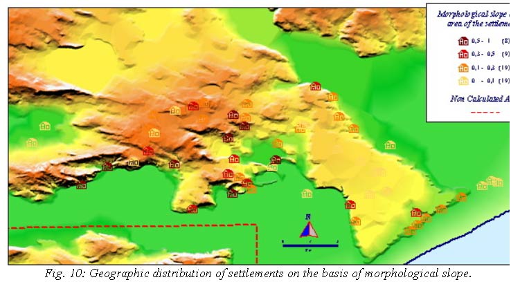
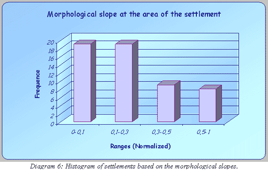
Figure 10 depicts the geographic distribution of the settlements in conjunction to the morphologic inclinations of the area and diagram 6 indicated the quantitative distribution of them on the basis of morphology. Finally, visibility analysis concluded that all the settlements dated A.D were visible from the area of Beziers.
Conclusions
The values of morphologic inclinations are generally low; the higher values are located in the southeastern part of the area and coincide with carbonate rocks.
In view of identifying the most possible cadastre in the area of Beziers, GIS and GPS technologies, remote sensing methods and statistics have been applied; the prevailing cadastre of the area is orientated N-S (358ο) and E-W (88ο). The average distances of the principal lines are 702m, 707m and 803m. The creation and the movement of possible grids concluded to the one that most of the lines (765) and most of the possible centuries (44) fall within. This grid corresponds to the orientation of 358ο and the distance of 707m and is concerned to represent a potential architectural arrangement of the ancient landscape. The results of the current research are in agreement with the results of the research of Clavel-Leveque (2002) that were produced with different methodology than the current one.
The analysis of the orientation of the linear elements belonging to the organization of the ancient landscape concluded that they coincide with the orientation of the physicogeographic characteristics of the area.
The combinatory study of the linear elements and the lithologic formations of the area returned that the presence of most of the settlements are on alluvial deposits and marles, well-justified since the biggest part of the area is covered from those formations.
The consideration of the linear elements in alliance with the morphology proved that most of the lines are located on the lowest range of morphologic inclinations’ values (0-0,3%).
The study of the archaeological data, settlements, identified and mapped with the combinatory use of GPS and GIS, together with the physicogeographic, geomorphologic and lithologic characteristics, points out that:
- Most of the settlements are located at low elevation values, lower than 20m, and on alluvial and marle rocks.
- In the beginning of 1st century B.C. a great amount of settlements are located at higher elevation values, up to 85m. The settlements keep increasing during the 1st century B.C. with a geographic distribution that includes all the altitudal ranges met in the area. Most of the sites are located on alluvial deposits and marles, such as in all cases, and an important number of them on carbonate rocks.
- In the two first centuries A.D. the settlements are increased along the coastal zone, while the 3rd century A.D. there is a decrease.
- During the 1st and the 2nd century A.D. most of the settlements are located up to the elevation of 35m. From the 3rd century A.D. there is a gradual decrease; the geographic distribution, however, regarding morphology and lithology.
The visibility analysis stressed out that most of the settlements dated A.D. are, undoubtedly, visible from the area of Beziers. Table 2 illustrates the percentage of visible settlements per period.
| Period | Percentage |
|---|---|
| 1st century B.C | 19,4 |
| 1st century A.D | 28,5 |
| 2nd century A.D | 28,5 |
| 3rd century A.D | 26,8 |
Bibliography
Clavel-Lévêque M., 1983, Cadastres et espace rural, Approches et réalités antiques, Paris, CNRS éditions, 1983, p. 9-13.
Clavel-Lévêque M., 1983a, « Paysages et cadastres antiques dans le Piscénois », Études sur l’Hérault, 1983, 14/5-6, p. 3-10.
Clavel-Lévêque M., 1983b, « Pratiques impérialistes et implantations cadastrales », Ktema, Civilisations de l’Orient, de la Grèce et de la Rome antiques, 8, 1983, p. 185-251.
Clavel-Lévêque M., 1988, « Résistance, révoltes et cadastres: problémes du contrôle de la terre en Gaule transalpine », in Forms of control and subordination in antiquity [Proceedings of the International symposium for studies on ancient worlds, January 1986, Tokyo], Toru Yuge et Masaoki Doi éd., Leiden, Brill, 1988, p. 177-208.
Clavel-Lévêque M., 1992, « Centuriation, géométrie et harmonie. Le cas du Biterrois », Mémoires, Centre Jean Palerne, 11, 1992 (Mathématiques dans l’antiquité), p. 161-176.
Clavel-Lévêque M., 1993, « Un plan cadastral à l’échelle. La forma de bronze de Lacimurga », Estudios de la Antigüedad, 6/7, 1993, p. 175-182.
Clavel-Lévêque M., Lorcin M.-T., Lemarchand G., Les campagnes françaises, précis d’histoire rurale, Paris, Éditions sociales, 1983, p. 7-106.
Chouquer G., Clavel-Lévêque M., « Des formes aux paysages. Quinze ans de recherches sur les cadastres antiques », Histoire de l’art, 1990, p. 91-96.
Clavel-Lévêque M., « Le réseau centurié Béziers A », Atlas Historique des Cadastres d’Europe II, Commission européenne (Luxembourg) Action COST G2. Paysages anciens et structures rurales, 2002, dossier 3, p. 1-12.
MapBasic, Troy/New York, MapInfo Corporation, 1999.
Akima H., « A method for bivariate interpolation and smooth surface fitting for irregulary distributed data points », ACM Transactions on Mathematical Software, 4/2, 1978, p. 148-159.
Aronoff S., Geographic Information Systems: A Management Perspective, Ottawa, 1989.
Avery T.E., Intrepretation of Aerial Photographs, Minneapolis, Burgess Publishing Company, 1973.
Burrough P.A.,. Geographical Information Systems for Natural Resources Assessment, New York, Oxford University Press, 1983.
Chrisman N.R.,. « Efficient Digitising Trough the Combination of Appropriate Hardware and Software for Error Detection and Editing », International Journal of Geographical Information Systems, 1, 1987, p. 265-277.
Clarke K.C., Analytical and Computer Cartography, Englewood Cliffs (N.J), Prentice-Hall, 1990.
Dana P.H., « Global Positioning System (GPS) Time Dissemination for Real-Time Applications », Real-Time Systems: The International Journal of Time Critical Computing Systems, 12/1, january 1997, p. 9-40.
Dana P.H., 1998a, « GPS: Positioning Techniques and Time and Frequency Dissemination », in Tecnología Sin Límite: XIII Simposium Internacional De Electrónica y Comunicaciones. ITESM, Monterrey, Mexico, 1998.
Dana P.H., 1998b, « Preliminary Mapping of Community Boundaries with GPS », in The Association of American Geographers 94th Annual Meeting, Boston, Massachusetts, 1998.
Dana P.H., Bruce P.Μ., « The Role of GPS in Precise Time and Frequency Dissemination », GPS World, july-august 1990. [On line] http://www.pdana.com/PHDWWW_files/gpsrole.pdf
Dangermond J.,. « A Classification of Software Components Commonly Used in Geographic Information Systems », Proceedings of the U.S.-Australia Workshop on the Design and Implementation of Computer- Based Geographic Information System, Honolulu, 1982, p. 70-91.
Demers M.N., Fundamental of Geographic Information Systems, John Wiley & Sons, 1997.
Evelpidou N., Geomorphological and Environmental study of Naxos island using Remote Sensing and GIS techniques, Thesis, 2001, 226 p.
Fotheringham S. et O’Kelly M., Spatial interaction models: Formulations and applications, Dordrecht, Kluwer Academic Publishers, 1989.
Goldberger A., « Best linear unbiased prediction in the generalized linear regression mode », l, JASA (Journal of the American statistical association), 57, 1962, p. 369-375.
Kaplan E. D., éd., Understanding GPS: Principles and Applications, Boston, Artech House Publishers, 1996.
Korshkariov A.V., Tikunov V.S. et Trifimov A.M., « The Current State and the Main Trends in the Development of Geographical Information Systems in the USSR », International Journal of Geographical Information Systems, 3/3, 1989, p. 257-272.
Lillesand T.M. et Kiefer R.W., Remote Sensing and Image Interpretation, New York, John Wiley & Sons, 1995.
MapInfo Professionnal, MapInfo Corporation, New York, Troy, 1998.
Marble D., Lauzon J.P. et Mc Granaghan M., « Development of a Conceptual Model of the Manual Digitizing Progress », Introductory Readings in Geographic Information Systems, D.J. Peuquet et D.F. Marle éds., Londres, 1990, p. 341-352.
Marble D.F. et Peuquet D.J.,. « Geographic Information Systems in Remote Sensing », Manual of Remote Sensing, 1, 2nd éd., R.N. Colwell éd., Falls Church, American Society of Photogrammetry, 1983, p. 923-957.
Rhind D.W., 1988, « A GIS Research Agenda. », International Journal of Geographical Information Systems, 2, 1988, p. 23-28.
Rhind D.W., 1992, « Data Access, Charging and Copyright and Their Implications for GIS », International Journal of Geographical Information Systems, 6/1, 1992, p. 13-30.
Snyder J.P.,. Map Projections. A Working Manual. U.S. Geological Survey, Professional Paper 1935, Washington DC, U.S. Government Printing Office,1988.
Tomlinson R.F., « Geographic Information Systems: The New Frontier », The Operational Geographer, 5, 1984, p. 31-35.
Vassilopoulos A., « The “cadastre Grid Software” to deduce possible Roman cadastre grids », Dialogues d’Histoire Ancienne, 25/1, 1999, p. 233-241.
Vertical Mapper, Northwood Geoscience Ltd., 1999.
Wastson, D. F., 1992, Contouring, Aguide to the Analysis and the Display of Spatial Data: Tarrytown, New York, Elsevier Science Inc., 321 pages.
Annexe
| Ranges of morphologic slopes (%) | Σ(length) possible lines of Roman cadastre per range of morphologic slopes | Percentage of the area represented by every morphologic slope (%) | Σ(length)/ occupied area of slope |
|---|---|---|---|
| 0 – 0,3 | 1.084,640 | 31,024 | 34.961 |
| 0,3 - 1 | 139,265 | 3,855 | 36.125 |
| 1 - 3 | 603,375 | 19,003 | 31.751 |
| 3 - 5 | 517,207 | 17,938 | 28.832 |
| 5 - 10 | 473,247 | 20,791 | 22.762 |
| 10 - 20 | 95,035 | 6,344 | 14.980 |
List of figures
Fig. 1. Geographical distribution of lithological formations, of abrupt changes of morphological slope and of archaeological sites (Wastson, 1992).
Fig. 2. Geographical distribution of average values % of morphological slope.
Fig. 3. Both lines indicating land divisions and, in general, lines deriving from human intervention, as well as lines of physical characteristics have been considered possible axes of Roman cadastre. The exact location of the lines was identified and recorded with the use of GPS during fieldwork.
Fig. 4. Geographic distribution of possible Roman cadastre lines on the basis of their orientation.
Fig. 5. Geographic distribution of lithological formations, of the relief and of possible Roman cadastre lines falling within the cadastre of orientation 358ο / distance axis 707 m.
Fig. 6. Geographic distribution of drainage basin’s branches in relation to their orientation.
Fig. 7. The archaeological settlements ( their exact location identified and recorded with the use of GPS during fieldwork) in relation to the physicogeographic characteristics.
Fig. 8. The archaeological settlements of the area, dated back from the Neolithic era up to modern times, in relation to the lithologic formations.
Fig. 9. Geographic distribution of settlements on the basis of elevation ranges, defined after having created relief’s interpolation in order to derive a more detailed presentation of the relief.
Fig. 10. Geographic distribution of settlements on the basis of morphological slope.
Fig. 11. The result of applying the algorithm “Viewshed” from the highest point of the study area.
Fig. 12. The picture depicts the simplest way of defining visibility from a specific point. Visible areas from the pre-defined point are coloured red, while non visible areas are coloured blue.
Fig. 13. Parts of the lines that have visibility or not can be represented by different colours on a thematic map (green and red respectively). The arrows of the lines indicate the view point.
Diagram 1. Algorithm’s response to the visibility analysis. The specific response regards the visibility from the highest point of a settlement.
Diagram 2. Histogram of linear elements of the study area based on their orientation.
Diagram 3. Distribution of possible Roman cadastre lines in conjunction with the morphological slopes of the area.
Diagram 4. Quantitative analysis of possible cadastre lines in conjunction with the axes of the drainage system.
Diagram 5. Distribution of settlements based on the relief.
Diagram 6. Histogram of settlements based on the morphological slopes.